Canonical Correlation Analysis Model

Canonical Correlation Analysis (CCA) was first proposed by Hotelling in 1936 [1]. Because CCA finds correlations between two multivariate data sets, CCA data structures are a good fit for exploring relationships between the input and output variables found in ensemble data sets (such as those generated for sensitivity studies, uncertainty quantification, model tuning, or parameter studies). Slycat™ uses CCA to model the many-to-many relationships between multiple input parameters and multiple output metrics. CCA is a linear method and a direct generalization of several standard statistical techniques, including Principal Component Analysis (PCA), Multiple Linear Regression (MLR), and Partial Least Squares (PLS) [2] [3].

CCA operates on a table of scalar data, where each column is a single input or output variable across all runs, and each row consists of the values for each of the variables in a single simulation. Slycat™ requires the number of rows (samples) to be greater than the minimum variable count of the inputs or the outputs. A more meaningful result will be obtained if the ratio of runs to variables is ten or more. Additionally, columns cannot contain the same value for all runs. Slycat™ will reject such columns from being included in the CCA analysis, since they contribute no differentiating information. CCA cannot handle rows with missing data, Inf, -Inf, NAN, or NULL values. Slycat™ will remove rows from the analysis if any of the values in either the input or output variable sets include such data. However, if the bad values are only in columns that are not analysis variables, the row will be used.

For a concise description of CCA, we need the following definitions. Given n samples (n rows in the table), the input variables (presumed to be independent) will be referred to as the set X = {x₁, …, x_n} and the output (dependent) variables as the set Y = {y₁, …, y_n}. Each vector x_i has p₁ components and each vector y_j has p₂ components. CCA attempts to find projections a and b such that R² = corr (a^TX, b^TY) is maximized, where corr (•,•) denotes the standard Pearson correlation.

The vectors a^TX and b^TY are known as the first pair of canonical variables. Further pairs of canonical variables are orthogonal and ordered by decreasing importance. In addition to the canonical variables, the R² value for each variable pair is obtained, and various statistics can be computed to determine the significance of the correlation. A common statistic used in this context is the p-value associated with Wilks’ λ [4]. Slycat™ provides both R² and p-values for each canonical component as part of the Correlation View (see the figure below). Note that these statistics assume that the data is normally distributed. If your data does not follow a normal distribution, be aware that these statistics will be suspect and adjust your interpretation of the results accordingly.

Once the canonical variables are determined, they can be used to understand how the variables in X are related to the variables in Y, although this should be done with some caution. The components of the vectors a and b can be used to determine the relative importance of the corresponding variables in X and Y. These components are known as canonical coefficients. However, the canonical coefficients are considered difficult to interpret and may hide certain redundancies in the data. For this reason, Slycat™ visualizes the canonical loadings, also known as the structure coefficients. The structure coefficients are generally preferred over the canonical coefficients because they are more closely related to the original variables. The structure coefficients are given by the correlations between the canonical variables and the original variables (e.g. corr (a^TX, X) and corr (a^TY, Y)). These are calculated using Pearson’s correlation between each column of X or Y and the corresponding canonical variable.

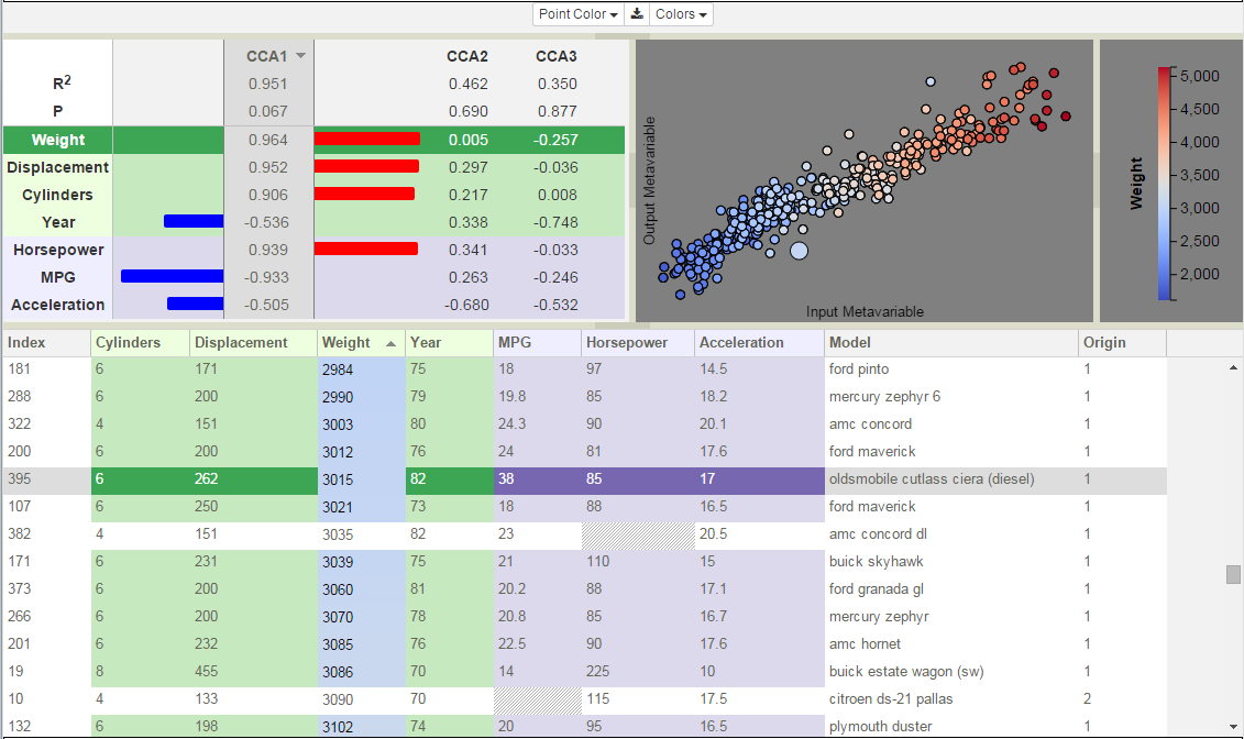
Canonical components are shown in the Correlation View in the upper left.

• Cars Example Data Set
• Creating a CCA Model
  • Local Files
  • Remote Files
  • Select Columns
  • Name Model
• CCA Model Visualization
  • Correlation View
  • Simulation View
    • Legend
    • Color-Coding Points
    • Selecting Points
  • Variable Table
    • Sorting
    • Variable Selection
    • Simulation Selection

Footnotes

[1]

Hotelling, H., Relations Between Two Sets of Variates. Biometrika, 28, 321-377 (1936).

[2]

Adams, B.M., Ebeida, M.S., Eldred, M.S., Jakeman, J.D., Swiler, L.P., Bohnhoff, W.J., Dalbey,K.R., Eddy, J.P., Hu, K.T., Vigil, D.M., Bauman, L.E., and Hough, P.D., Dakota, a Multilevel Parallel Object-Oriented Framework for Design Optimization, Parameter Estimation, Uncertainty Quantification, and Sensitivity Analysis: Version 5.3.1 User’s Manual. Tech. Rep. SAND2010-2183, Sandia National Laboratories (2013).

[3]

Ayachit, U., Bauer, A., Geveci, B., O’Leary, P., Moreland, K., Fabian, N., and Mauldin, J., ParaView Catalyst: Enabling In Situ Data Analysis and Visualization, Proceedings of the First Workshop on In Situ Infrastructures for Enabling Extreme-Scale Analysis and Visualization (ISAV2015), pp. 25-29, ACM, New York, NY (2015).

[4]

Krzanowski, W. J., Principles of Multivariate Analysis. A User’s Perspective. Oxford University Press, London (1988).