Scatterplot View
The Scatterplot View represents each ensemble member as a point in a two-dimensional plot, where the variables that are used for the x-axis, y-axis, and point color-coding are interactively selected. As with the CCA Model, when individual points or groups of points are selected within the plot (see Selecting Points), corresponding rows in the Variable Table are simultaneously selected, and vice versa.
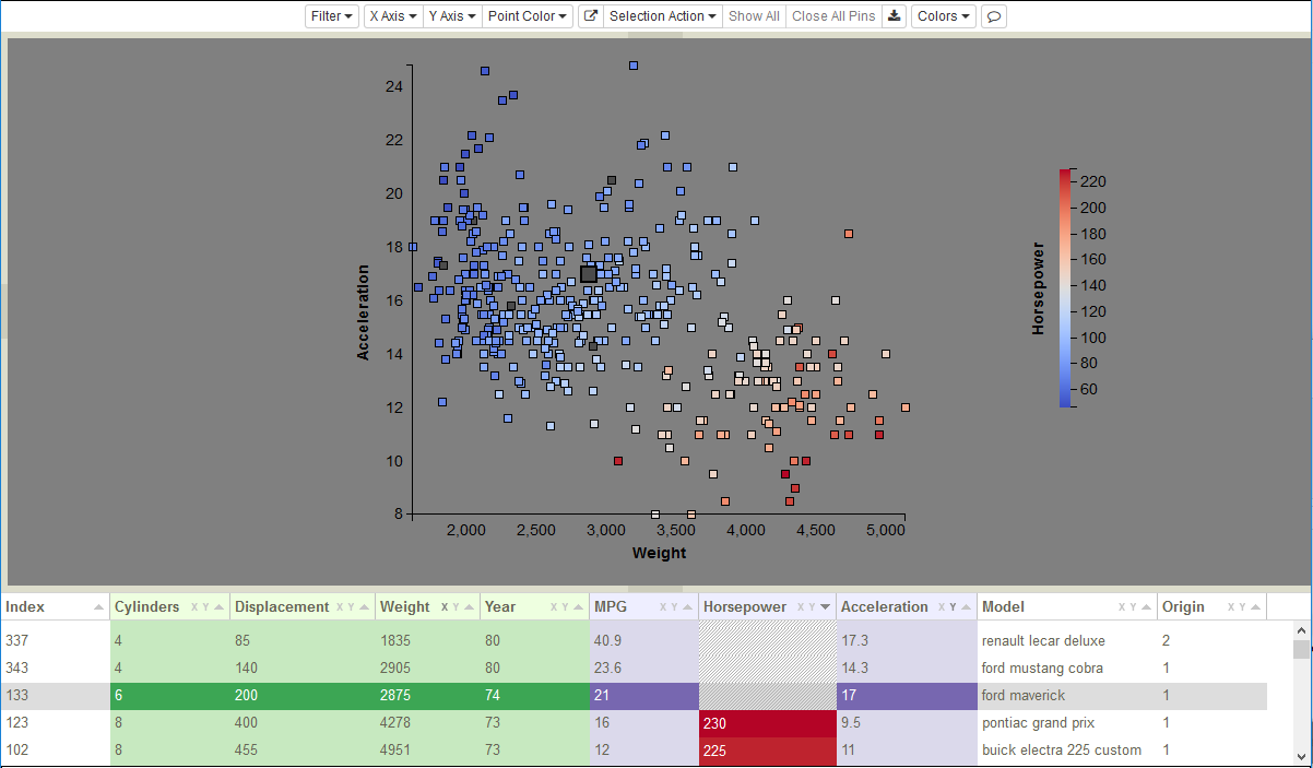
Figure 27: Parameter Space Model visualization of the Cars data set.
However, the Parameter Space Model’s Scatterplot View possesses additional capabilities that the CCA Model’s Simulation View lacks. If the Variable Table contains media columns (URIs for images, videos, time series tables, or STLs), hovering over a point with the mouse can be used to retrieve media items from remote HPC systems. The media variable to be retrieved is selected through a Media Set dropdown list, which only appears in the controls (as shown in Figure 28) when media columns are present in the table.

Figure 28: Full set of Parameter Space model-specific controls.
Another key feature in the Scatterplot View is the ability to reduce the number of visible points through filtering or point hiding. This is important for interacting with large ensembles, since point overlap and occlusion increase with ensemble size. Additionally, the Scatterplot View enables the inclusion of points with missing data. Although a point still requires values to exist in both axis variables to define its coordinates, none of the other variables need to have a value for the point to be displayed. The points colored dark gray in Figure 27 are examples of rows with missing values for Horsepower. One of these is row 133, which is highlighted in both the scatterplot (enlarged point) and the table (darkened row).